The AI Deployment Playbook

Open models such as GPT-OSS, Whisper V3, DeepSeek, and Gemma continue to raise the ceiling for what compound AI systems can do.

Each release arrives with more capability, but adoption depends on how ready the surrounding stack is — support libraries, inference frameworks, and the team’s own budget priorities.

These updates stretch deployment pipelines beyond their design. Infrastructure that once managed smaller models now meets longer contexts and changes GPU behavior across versions.

If your model deployment still runs below 60% GPU utilization, this playbook will show you where your budget is leaking.

Why is deploying large models still painful?

McKinsey estimates global compute infrastructure spending could reach $6.7 trillion by 2030, driven primarily by AI workloads. Yet many production pipelines still operate at under 60 percent utilization, with latency that fluctuates beyond acceptable service levels.

The pain comes from architecture that hasn’t caught up with model complexity. As context windows extend and inference frameworks evolve, older systems reveal failure points that demand custom fixes.

• Memory becomes fragmented as sequences extend beyond expected limits

• Kernel performance slows when precision modes switch during execution

• KV-cache coordination fails when GPUs carry uneven workloads

• Framework updates drift away from hardware and driver compatibility

• Scaling logic inflates cost long before it delivers usable throughput gains

Each of these reflects a deeper coordination problem — models and infrastructure evolving at different speeds.

What drives up deployment cost and latency?

Most teams blame GPU choice or model size. In reality, the biggest costs hide in how workloads are shaped and scheduled.

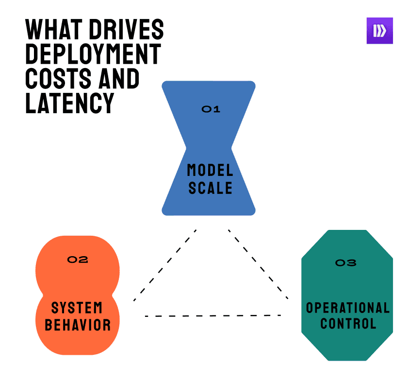
Large-model deployment is less about how powerful your hardware is — and more about how intelligently you use what you already have.

You can think of cost as a triangle between model scale, system behavior, and operational control. Each side exerts pressure on the others.

When any one of these moves faster than the others, instability follows. That’s why scaling a model 2× rarely doubles cost — it multiplies inefficiency unless the scheduler, cache logic, monitoring stack, and the team’s operational rhythm evolve in sync.

In short: cost is a symptom of misalignment, just like any DevOps or MLOps system where coordination breaks before capacity does.

Engineering the Layer Between Frameworks and Scale

1. Understanding how the workload really behaves

Teams often lean on model specs to predict performance. Parameters and context length look like they tell the story. In production, they rarely do. Once a model runs at scale, its behavior drifts for reasons those specs never describe.

Workloads move with the data that hits them. A slight change in input shape, batch size, or cache state can skew latency in ways that seem random. Context growth fragments memory. Precision drift slows kernels. Cache desync leaves response times uneven.

These are just some of the things that can be surfaced with the right tools and metrics. Tools like vLLM, TGI, or SGLang profilers though visibility fades fast once workloads scale beyond a single node.

2. Mapping the moving parts

Once you start measuring how a workload behaves, the next challenge is mapping that behavior to infrastructure decisions.

In practice, a system has to navigate trade-offs across:

• Cache vs. compute locality — where does your KV-cache live vs. where your token computation runs?

• Batch shaping and packing — how many tokens or requests per batch, and how tightly they can be packed without starving some GPUs.

• Parallelism strategy — data parallelism, tensor parallelism, or mixtures, depending on model structure and hardware topology.

• Load balancing and autoscaling — distributing traffic dynamically across nodes and scaling up/down without creating hotspots.

In a smart workflow orchestration, these pieces are decoupled yet coordinated: the system can swap out caching layers, pick among parallelism strategies, or adjust batch-routing policies depending on workload signals

When done well, the orchestration layer acts like a chess master: given the workload’s runtime signature, it picks which component goes where, when, and how — continuously.

3. Rebuilding control without rebuilding everything

Each inference framework handles one layer of the problem well but leaves coordination to the team. As models grow and pipelines expand, the gap between framework-level tuning and full-system control becomes the real cost center.

4. Tuning for feedback with dynamic settings

Static settings tend to age fast because workloads never stay constant. As batch size, cache policy, and parallelism levels drift with traffic patterns, configurations that once worked start creating latency instead of reducing it.

Systems that ignore this drift lose predictability long before they exhaust compute.

A simple feedback loop keeps the stack aligned with live conditions. It watches key runtime signals and adjusts system behavior as they shift:

• The batch size decreases when tail latency begins to rise.

• Cache memory is rebalanced when reuse drops below expected thresholds.

• Workloads move between GPUs when utilization tilts unevenly.

• Decoding thresholds update automatically when throughput begins to decline.

These adjustments happen continuously. The result is a system that stays stable without constant returning or manual intervention.

Metrics to Track Model Deployment

Each model family places different pressure on the system. Tracking the right signals keeps scaling measurable and makes performance easier to manage.

In practice, these signals come from profiler hooks, GPU telemetry, and framework metrics such as Triton’s Prometheus exporter or vLLM’s runtime profiler. Custom tracing at the model API layer fills in the remaining blind spots.

When these measurements are viewed together, they reveal where performance lacks and how scaling responds under real traffic.

Once the data holds steady, deployments behave consistently. They turn into systems that teams can adjust with intent and predict with confidence.

Re-asses Your Latency and Cost Compromises

Curious where you’re losing money and time in your current deployment setup?

Most teams overpay for inference without realizing it. Run a workload benchmark with Pipeshift and see how much GPU time you’re wasting. You’ll walk away with a clear view of what to fix and what to keep.

Start optimizing today — book a call.